![]()
You can run this notebook in a live session or view it on Github.
Introduction to Xoak#
This notebook briefly shows how to use Xoak with Xarray’s advanced indexing to perform point-wise selection of irrelgularly spaced data encoded in coordinates with an arbitrary number of dimensions (1, 2, …, n-d).
Note: Xoak relies on xarray.indexes.NDPointIndex, which has been added in Xarray version 2025.07.1.
[1]:
import matplotlib.pyplot as plt
import numpy as np
import xarray as xr
import xoak

xr.set_options(display_expand_indexes=True);
Let’s first create an xarray.Dataset of latitude / longitude points located randomly on the sphere, forming a 2-dimensional (x, y) model mesh (note that Xoak supports indexing coordinates with an arbitrary number of dimensions).
[2]:
shape = (100, 100)
lat = np.random.uniform(-90, 90, size=shape)
lon = np.random.uniform(-180, 180, size=shape)

field = lat + lon
[3]:
ds_mesh = xr.Dataset(
    coords={'lat': (('x', 'y'), lat), 'lon': (('x', 'y'), lon)},
    data_vars={'field': (('x', 'y'), field)},
)

ds_mesh
[3]:
<xarray.Dataset> Size: 240kB
Dimensions:  (x: 100, y: 100)
Coordinates:
    lat      (x, y) float64 80kB -42.21 68.76 -27.52 ... 30.89 -76.7 41.37
    lon      (x, y) float64 80kB 44.8 90.71 139.0 -81.45 ... -52.4 120.7 -169.8
Dimensions without coordinates: x, y
Data variables:
field (x, y) float64 80kB 2.592 159.5 111.5 -169.1 ... -21.5 44.03 -128.4We first need to build an index to allow fast point-wise selection. Xoak extends xarray.indexes.NDPointIndex with different structures available for use cases depending on the data. In the example below we use a wrapper around sklearn.BallTree using the Haversine distance metric that is suited for indexing latitude / longitude points.
With this index, it is important to specify lat and lon in this specific order. Both the lat and lon coordinates must have exactly the same dimensions in the same order, here ('x', 'y').
[4]:
ds_mesh = ds_mesh.set_xindex(
    ['lat', 'lon'],
    xr.indexes.NDPointIndex,
    tree_adapter_cls=xoak.SklearnGeoBallTreeAdapter
)

ds_mesh
[4]:
<xarray.Dataset> Size: 240kB
Dimensions:  (x: 100, y: 100)
Coordinates:
  * lat      (x, y) float64 80kB -42.21 68.76 -27.52 ... 30.89 -76.7 41.37
  * lon      (x, y) float64 80kB 44.8 90.71 139.0 -81.45 ... -52.4 120.7 -169.8
Dimensions without coordinates: x, y
Data variables:
    field    (x, y) float64 80kB 2.592 159.5 111.5 -169.1 ... -21.5 44.03 -128.4
Indexes:
  ┌ lat      NDPointIndex (SklearnGeoBallTreeAdapter)
└ lonLet’s create another xarray.Dataset of latitude / longitude points that here correspond to a trajectory on the sphere.
[5]:
ds_trajectory = xr.Dataset({
    'latitude': ('trajectory', np.linspace(-10, 40, 30)),
    'longitude': ('trajectory', np.linspace(-150, 150, 30))
})

ds_trajectory
[5]:
<xarray.Dataset> Size: 480B
Dimensions:    (trajectory: 30)
Dimensions without coordinates: trajectory
Data variables:
    latitude   (trajectory) float64 240B -10.0 -8.276 -6.552 ... 38.28 40.0
longitude (trajectory) float64 240B -150.0 -139.7 -129.3 ... 139.7 150.0We can now simply use xarray.Dataset.sel() to select the mesh points that are the closest to the trajectory vertices. All indexer coordinates (latitude and longitude in this example) must have the exact same dimensions (here 'trajectory'). Indexers must be given for each coordinate used to build the index above, (here latitude for lat and longitude for lon).
[6]:
ds_selection = ds_mesh.sel(
    lat=ds_trajectory.latitude,
    lon=ds_trajectory.longitude,
    method="nearest",
)

ds_selection
[6]:
<xarray.Dataset> Size: 720B
Dimensions:  (trajectory: 30)
Coordinates:
    lat      (trajectory) float64 240B -11.07 -7.522 -8.947 ... 37.51 37.61 39.5
    lon      (trajectory) float64 240B -150.0 -139.6 -129.5 ... 140.3 150.6
Dimensions without coordinates: trajectory
Data variables: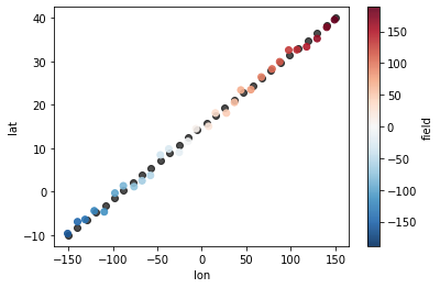
field (trajectory) float64 240B -161.1 -147.1 -138.4 ... 177.9 190.1Let’s plot the trajectory vertices (black dots) and the resulting selection (dots colored by the field values):
[7]:
fig, ax = plt.subplots()
ds_trajectory.plot.scatter(ax=ax, x='longitude', y='latitude', c='k', alpha=0.7)
ds_selection.plot.scatter(ax=ax, x='lon', y='lat', hue='field', alpha=0.9);
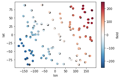
Xarray also supports providing coordinates with an arbitrary number of dimensions as indexers, like in the example below with vertices of another mesh on the sphere.
[8]:
ds_mesh2 = xr.Dataset({
    'latitude': (('x', 'y'), np.random.uniform(-90, 90, size=(10, 10))),
    'longitude': (('x', 'y'), np.random.uniform(-180, 180, size=(10, 10)))
})

ds_selection = ds_mesh.sel(
    lat=ds_mesh2.latitude,
    lon=ds_mesh2.longitude,
    method="nearest",
)

ds_selection
[8]:
<xarray.Dataset> Size: 2kB
Dimensions:  (x: 10, y: 10)
Coordinates:
    lat      (x, y) float64 800B -38.96 -82.12 -68.52 ... 82.12 -34.42 8.725
    lon      (x, y) float64 800B 134.5 135.9 -90.68 124.3 ... 149.9 -67.84 10.59
Dimensions without coordinates: x, y
Data variables:
field (x, y) float64 800B 95.52 53.81 -159.2 94.13 ... 232.0 -102.3 19.31[9]:
fig, ax = plt.subplots()
ds_mesh2.plot.scatter(ax=ax, x='longitude', y='latitude', c='k', alpha=0.7)
ds_selection.plot.scatter(ax=ax, x='lon', y='lat', hue='field', alpha=0.9);
[ ]: